flowchart LR
    I["Carbon Information"]
    A["Environmental Concern"]
    D["Downsizing Choice"]
    I --> A
    A --> D
Lecture 11 - Causal Inference Methods
ENCI707: Engineering Demand and Policy Analysis
Learning Objectives
- Understand why choice modellers should care about causal inference
- Explain the three sources of causal identification
- Connect causal identification sources to tools
- Incorporate causal identification tools into choice model specifications
Why Choice Modellers Should Care About Causal Inference
Traditional choice studies estimate \[P(y_i=j|X_i)\]
But policymakers usually ask ``what would happen if we changed X?”
- This is a counterfactual question, not about prediction or goodness-of-fit
Returning to our previous example: People who like transit move near transit & ride transit
- We observe transit-proximate home choice & transit use choice but the real story is transit preference
Three Sources of Causal Identification
- Randomization to create comparability - e.g., random treatment in DCE
- Statistical adjustment to control for observed confounders
- Matching
- Propensity scores (PS)
- Regression
- Natural experiments by exploiting external variation
- Instrumental variables (IV)
- Difference-in-differences (DiD)
- Regression discontinuity design (RDD)
Transportation Examples
Propensity Score Matching for TOD Choice
- Policy question: Does living near transit increase transit use?
- Problem: People are not randomly assigned to neighbourhoods
- Matching on confounders: Find people who are similar on income, household size, age, employment, and vehicle ownership but differ on transit proximity
- Option 1: Estimate the model using a sample filtered to include only matched samples
- Option 2: Use inverse propensity score weights directly in the choice model - i.e., \(w_i = \frac{T_i}{e_i} + \frac{1-T_i}{1-e_i}\) where \(e_i = P(T_i=1|X_i)\)
IV for Residential Self-Selection
- Policy question: Does living near transit increase transit use?
- Problem: if \(U_{Transit} = \beta N + \varepsilon\) where \(N\) is a binary treatment for living near transit and we omit transit preference then \(Cov(N,\varepsilon)\neq0\)
- IV solution: use 2-stage control function estimation to adjust for endogeneity bias
- \(N = \pi Z + \nu\) where \(Z\) is an instrument - e.g., historical streetcar network
- \(Z\) affects whether someone lives near transit today but does not directly affect current transit use
- \(U_{Transit} = \beta N + \lambda \hat{\nu} + \varepsilon\)
- \(\hat{\nu}\) is the residual part of residential location that could be related to transit preference
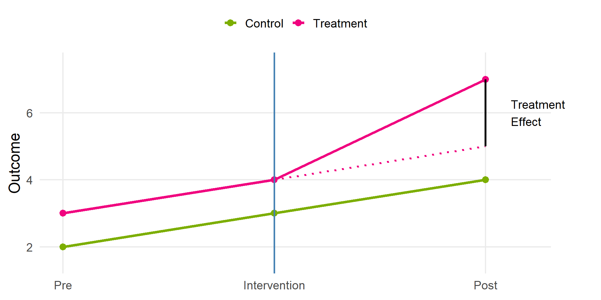
DiD for New Rail Line
- Policy question: Did a new rail line increase transit ridership?
- Problem: need a counterfactual trend for before-after case
- DiD solution: \(U_{Transit,nt} = \beta X_{nt} + \delta (RailArea_n\times Post_t) + \varepsilon_{nt}\)
- \(\delta\) measures the DiD treatment effect
- Requires panel data
- Can include heterogeneity via \(\delta_i\) and panel mixed logit model
Mediation for Carbon Information->Attitude->Housing Downsizing
- Policy question: Does information affect residential choice?
- Problem: need to capture information->attitude connection
- \(U_{ni} = \beta Size_i + \gamma Carbon_i +\varepsilon_{ni}\)
- Tells use whether carbon information matters but not why
- ICLV solution: Mediation structure
- Carbon information changes latent environmental concern, which changes residential preference
Illustrating the 4 Methods
PS
%%{init: {'theme': 'base', 'themeVariables': { 'fontSize': '12px' }}}%%
flowchart TB
    P["Income, Age, <br>Household Characteristics"] --> N["Transit Proximity"]
    P --> T["Transit Mode Choice"]
    N --> T
IV
%%{init: {'theme': 'base', 'themeVariables': { 'fontSize': '12px' }}}%%
flowchart LR
    Z["Streetcar<br>Network"] --> N["Lives Near<br>Transit"]
    N --> T["Transit Use"]
    V["Residual ν"] --> T
DiD
%%{init: {'theme': 'base', 'themeVariables': { 'fontSize': '12px' }}}%%
flowchart TB
    T["Treatment <br>(Near Stations)"] --> B1["Before"]
    T --> A1["After"]
    C["Control <br>(Far Stations)"] --> B2["Before"]
    C --> A2["After"]
Mediation ICLV Model
%%{init: {'theme': 'base', 'themeVariables': { 'fontSize': '12px' }}}%%
flowchart LR
    I["Carbon Info"] --> A["Environmental <br>Concern"]
    A --> Q["Indicators <br>(Q1-Q3)"]
    A --> U["Downsizing <br>Utility"] --> C["Housing <br>Choice"]
Supplemental Additional Details on Methods
Propensity Score Matching (PSM)
- Matching: restructure data for statistical analysis
- Goal is to create attribute balance between treatment & control samples
- Five step procedure
PSM: Step 1 - Define confounders & estimand
- Based on relevant literature
- Typically adjust control group to match treated to estimate effect of the treatment on the treated
- Careful! Including additional covariates may increase bias away from the true estimate if not all confounding covariates are available – avoid potential instrumental variables
PSM: Step 2 - Estimating propensity score
- Model of Pr(receiving treatment)
- Typically, a logistic regression for binary treatment, then use propensity score as covariate summary
- Propensity score gives a distance metric
PSM: Step 3 - Matching to restructure data
- Create matched pairs with control samples with closest propensity score – can be with/without replacement
- Better matches with replacement but may overuse some sample units
PSM: Step 4 - Diagnostics for balance & overlap
- Several diagnostics exist based on difference of means, etc.
- Evaluate and change model or method (if required)
PSM: Step 5 - Estimate treatment effect using restructured data
- Estimate regression model with propensity score and confounder variables
- Incorporate data restructuring via weights – typically inverse probability weights
Instrumental Variable (IV)
- When ignorability of treatment seems weak, IV can be a good approach
- Instrument \(z\) should predict the treatment \(T\) but not the outcome \(y\)
- Assumptions:
- Ignorability of instrument
- Monotonicity
- Nonzero association between treatment & instrument
- Exclusion restriction – no instrument effect on excluded variables
IV in Regression
- General framework \[𝑦_𝑖=\beta_0+\beta_1 𝑇_𝑖+\epsilon_𝑖\] \[𝑇_𝑖=\gamma_0+\gamma_1 𝑧_𝑖+𝜈_𝑖\]
- Where \(𝑧_𝑖\) is uncorrelated with both \(\epsilon_𝑖\) and \(𝜈_𝑖\) (ignorability and exclusion restriction)
- Identifiability: whether data contain sufficient information for unique estimation of parameter (or set of parameters)
IV in Regression
- With \[𝑦=\beta_0+\beta_1 𝑇+\beta_2 𝑧+𝑒𝑟𝑟𝑜𝑟\] \[𝑇=\gamma_0+\gamma_1 𝑧+𝑒𝑟𝑟𝑜𝑟\]
- Substituting \(T\) into \(y\): \[𝑦=(\beta_0+\beta_1 \gamma_0 )+(\beta_1 \gamma_1+\beta_2 )𝑧+𝑒𝑟𝑟𝑜𝑟\]
- where \(\beta_1\) is our parameter of interest
- Using \(𝑦=\delta_0+\delta_1 𝑧+𝑒𝑟𝑟𝑜𝑟\) where \(\delta_1=\beta_1 \gamma_1+\beta_2\) we get \[\beta_1=(\delta_1−\beta_2)/\gamma_1\]
IV in Regression
- Cannot estimate \(\beta_2\) because error in \(f(y)\) can be correlated with T – exclusion restriction means \(\beta_2=0\) giving \(\beta_1=\delta_1/\gamma_1\)
- Estimation is by two-stage least squares (2SLS)
- Standard errors require adjustment in instrumental variable estimation – should be accounted for in any software package
Exclusion Restriction Plausibility
- One way to assess the plausibility of the exclusion restriction is to calculate an estimate within a sample that would not be expected to be affected by the instrument
- Researchers estimated the effect of military service on earnings (and other outcomes) using, as an instrument, the lottery number for young men eligible for the draft during the Vietnam War
- Randomly assigned number and strongly affected the probability of military service
- Men with low lottery numbers may have altered their educational plans to avoid or postpone military service (would void exclusion restriction)
- Ran IV model for a sample of men who were assigned numbers so late that the war ended before they ever had to serve
- No clear relation between lottery number and earnings, providing support for the exclusion restriction
Weak Instrument
- Only assumption we can test – instrument has non-zero correlation with treatment variable
- If low correlation, then a weak instrument
Regression Discontinuity
- Non-random assignment but mechanism entirely known to researcher
- Consider a policy that gives tutoring to students with test scores < 60
- Consider all students with score in range of 60 – discontinuity at 60
- Works well when discontinuity relates to outcome – e.g., pre-test scores on post-test scores
- Does not work well if comparing across geography due to spatial heterogeneity
Fixed Effect Models
- Use repeated observations within groups – e.g., twin comparisons that holds confounding variables fixed
- Simply a regression model with group-specific intercepts \[𝑦_{𝑖𝑗}=\beta_0+\tau z_{𝑖𝑗}+\alpha_𝑖+\varepsilon_{𝑖𝑗}\]
- where \(j\) is an indicator of intra-group units
- Requires treatment to vary within groups
Difference-In-Differences
- Comparison across units (typically) using time as an additional dimension of variation
- E.g., effect of new school busing program on housing prices in school district
- Compare prices before/after between district with school busing program and those without it
- A measure of differences in trajectory